# Import necessary libraries
import numpy as np
import pandas as pd
import matplotlib.pyplot as plt
import seaborn as sns
from sklearn.model_selection import train_test_split
from sklearn.linear_model import Lasso, Ridge, LinearRegression
from sklearn.preprocessing import StandardScaler
from sklearn.metrics import mean_squared_error, r2_score
from sklearn.model_selection import cross_val_score
import warnings
warnings.filterwarnings('ignore')

# Set random seed for reproducibility
np.random.seed(42)

# Configure plotting

plt.rcParams['figure.figsize'] = (10, 6)Assignment: Lasso and Sparse Linear Model Recovery
Machine Learning
1 Introduction
In this assignment, you will explore the ability of the Lasso (Least Absolute Shrinkage and Selection Operator) to recover non-zero coefficients in sparse linear models. We’ll compare it with Ridge regression to understand their different behavior in feature selection.
1.1 Background
In many real-world applications, we have datasets with many features (p) but only a few are truly relevant. This is called a sparse setting. Lasso is particularly useful here because it can set coefficients to exactly zero, effectively performing feature selection.
2 Setup and Imports
3 Data Generating Process (DGP)
We’ll create a sparse linear model where only a few predictors have non-zero coefficients.
# Set parameters for the data generating process
n_samples = 200        # Number of observations
n_features = 50        # Total number of features
n_informative = 10      # Number of features with non-zero coefficients
noise_level = 1.0       # Standard deviation of the noise

# Generate feature matrix X
# Each column is a feature drawn from standard normal distribution
X = np.random.randn(n_samples, n_features)

# Create the true coefficient vector (beta)
# Most coefficients are zero (sparse model)
true_coefficients = np.zeros(n_features)

# Randomly select which features will have non-zero coefficients
informative_features = np.random.choice(n_features, n_informative, replace=False)
print(f"True informative features indices: {sorted(informative_features)}")

# Assign non-zero values to selected coefficients
# Values are drawn from a normal distribution with larger variance
for idx in informative_features:
    true_coefficients[idx] = np.random.randn() * 3

# Generate the response variable Y
# Y = X * beta + noise
Y = X @ true_coefficients + np.random.randn(n_samples) * noise_level

# Save the data and true coefficients for later analysis
data_dict = {
    'X': X,
    'Y': Y,
    'true_coefficients': true_coefficients,
    'informative_features': informative_features
}

# Create a DataFrame to better visualize the coefficients
coef_df = pd.DataFrame({
    'feature_index': range(n_features),
    'true_coefficient': true_coefficients
})

# Show the non-zero coefficients
print("\nNon-zero coefficients:")
print(coef_df[coef_df['true_coefficient'] != 0])
True informative features indices: [np.int64(0), np.int64(2), np.int64(4), np.int64(10), np.int64(15), np.int64(17), np.int64(19), np.int64(23), np.int64(44), np.int64(45)]
Non-zero coefficients:
feature_index true_coefficient
0 0 -5.038946
2 2 -2.678609
4 4 -1.823795
10 10 -1.610677
15 15 -2.561768
17 17 0.393326
19 19 1.786967
23 23 5.059156
44 44 -0.493334
45 45 5.9336214 Train-Test Split
Split the data into training and testing sets to evaluate model performance.
# Split the data into training and testing sets
# We use 70% for training and 30% for testing
X_train, X_test, Y_train, Y_test = train_test_split(
    X, Y, test_size=0.3, random_state=42
)

print(f"Training set size: {X_train.shape}")
print(f"Test set size: {X_test.shape}")

# Standardize the features (important for regularized regression)
# Fit the scaler on training data and apply to both train and test
scaler = StandardScaler()
X_train_scaled = scaler.fit_transform(X_train)
X_test_scaled = scaler.transform(X_test)
Training set size: (140, 50)
Test set size: (60, 50)5 Implementing Lasso Regression
5.1 Understanding Lasso
Lasso adds an L1 penalty to the ordinary least squares objective:
\[\min_{\beta} \frac{1}{2n} ||Y - X\beta||_2^2 + \alpha ||\beta||_1\]
where: - \(\alpha\) is the regularization parameter - \(||\beta||_1 = \sum_{j=1}^p |\beta_j|\) is the L1 norm
# Define different alpha values to test
# Alpha controls the strength of regularization
alphas = [0.0001, 0.001, 0.01, 0.1, 0.5, 1.0]

# Store results for each alpha
lasso_results = {}

for alpha in alphas:
    # Create and fit Lasso model
    # max_iter: maximum number of iterations for optimization
    lasso = Lasso(alpha=alpha, max_iter=10000)
    lasso.fit(X_train_scaled, Y_train)

    # Make predictions
    Y_train_pred = lasso.predict(X_train_scaled)
    Y_test_pred = lasso.predict(X_test_scaled)

    # Calculate metrics
    train_mse = mean_squared_error(Y_train, Y_train_pred)
    test_mse = mean_squared_error(Y_test, Y_test_pred)
    train_r2 = r2_score(Y_train, Y_train_pred)
    test_r2 = r2_score(Y_test, Y_test_pred)

    # Count non-zero coefficients
    n_nonzero = np.sum(lasso.coef_ != 0)

    # Store results
    lasso_results[alpha] = {
        'model': lasso,
        'coefficients': lasso.coef_,
        'train_mse': train_mse,
        'test_mse': test_mse,
        'train_r2': train_r2,
        'test_r2': test_r2,
        'n_nonzero_coef': n_nonzero
    }

    print(f"\nAlpha = {alpha}")
    print(f"  Non-zero coefficients: {n_nonzero}")
    print(f"  Train MSE: {train_mse:.4f}, Test MSE: {test_mse:.4f}")
    print(f"  Train R²: {train_r2:.4f}, Test R²: {test_r2:.4f}")
Alpha = 0.0001
  Non-zero coefficients: 50
  Train MSE: 0.6324, Test MSE: 1.4795
  Train R²: 0.9952, Test R²: 0.9872

Alpha = 0.001
  Non-zero coefficients: 50
  Train MSE: 0.6324, Test MSE: 1.4605
  Train R²: 0.9952, Test R²: 0.9874

Alpha = 0.01
  Non-zero coefficients: 49
  Train MSE: 0.6408, Test MSE: 1.3003
  Train R²: 0.9951, Test R²: 0.9888

Alpha = 0.1
  Non-zero coefficients: 19
  Train MSE: 0.9011, Test MSE: 1.0314
  Train R²: 0.9931, Test R²: 0.9911

Alpha = 0.5
  Non-zero coefficients: 8
  Train MSE: 3.3757, Test MSE: 3.0970
  Train R²: 0.9743, Test R²: 0.9733

Alpha = 1.0
  Non-zero coefficients: 8
  Train MSE: 8.9801, Test MSE: 9.0886
  Train R²: 0.9316, Test R²: 0.9216
6 Implementing Ridge Regression
6.1 Understanding Ridge
Ridge adds an L2 penalty to the ordinary least squares objective:
\[\min_{\beta} \frac{1}{2n} ||Y - X\beta||_2^2 + \alpha ||\beta||_2^2\]
where: - \(||\beta||_2^2 = \sum_{j=1}^p \beta_j^2\) is the squared L2 norm
# Store Ridge results for comparison
ridge_results = {}

for alpha in alphas:
    # Create and fit Ridge model
    ridge = Ridge(alpha=alpha)
    ridge.fit(X_train_scaled, Y_train)

    # Make predictions
    Y_train_pred = ridge.predict(X_train_scaled)
    Y_test_pred = ridge.predict(X_test_scaled)

    # Calculate metrics
    train_mse = mean_squared_error(Y_train, Y_train_pred)
    test_mse = mean_squared_error(Y_test, Y_test_pred)
    train_r2 = r2_score(Y_train, Y_train_pred)
    test_r2 = r2_score(Y_test, Y_test_pred)

    # For Ridge, count "effectively zero" coefficients (very small)
    threshold = 0.001
    n_small = np.sum(np.abs(ridge.coef_) < threshold)

    # Store results
    ridge_results[alpha] = {
        'model': ridge,
        'coefficients': ridge.coef_,
        'train_mse': train_mse,
        'test_mse': test_mse,
        'train_r2': train_r2,
        'test_r2': test_r2,
        'n_small_coef': n_small
    }

    print(f"\nAlpha = {alpha}")
    print(f"  Coefficients < {threshold}: {n_small}")
    print(f"  Train MSE: {train_mse:.4f}, Test MSE: {test_mse:.4f}")
    print(f"  Train R²: {train_r2:.4f}, Test R²: {test_r2:.4f}")
Alpha = 0.0001
  Coefficients < 0.001: 0
  Train MSE: 0.6324, Test MSE: 1.4816
  Train R²: 0.9952, Test R²: 0.9872

Alpha = 0.001
  Coefficients < 0.001: 0
  Train MSE: 0.6324, Test MSE: 1.4816
  Train R²: 0.9952, Test R²: 0.9872

Alpha = 0.01
  Coefficients < 0.001: 0
  Train MSE: 0.6324, Test MSE: 1.4812
  Train R²: 0.9952, Test R²: 0.9872

Alpha = 0.1
  Coefficients < 0.001: 0
  Train MSE: 0.6324, Test MSE: 1.4778
  Train R²: 0.9952, Test R²: 0.9873

Alpha = 0.5
  Coefficients < 0.001: 0
  Train MSE: 0.6343, Test MSE: 1.4666
  Train R²: 0.9952, Test R²: 0.9873

Alpha = 1.0
  Coefficients < 0.001: 1
  Train MSE: 0.6402, Test MSE: 1.4614
  Train R²: 0.9951, Test R²: 0.9874
7 Visualizing Coefficient Recovery
Let’s visualize how well each method recovers the true coefficients.
# Select a specific alpha for detailed comparison
selected_alpha = 0.1

# Get the coefficients for the selected alpha
lasso_coef = lasso_results[selected_alpha]['coefficients']
ridge_coef = ridge_results[selected_alpha]['coefficients']

# Create comparison plots
fig, axes = plt.subplots(2, 2, figsize=(15, 12))

# Plot 1: Lasso coefficients vs True coefficients
ax1 = axes[0, 0]
ax1.scatter(true_coefficients, lasso_coef, alpha=0.6)
ax1.plot([-5, 5], [-5, 5], 'r--', label='Perfect recovery')
ax1.set_xlabel('True Coefficients')
ax1.set_ylabel('Lasso Coefficients')
ax1.set_title(f'Lasso Coefficient Recovery (α={selected_alpha})')
ax1.legend()
ax1.grid(True, alpha=0.3)

# Plot 2: Ridge coefficients vs True coefficients
ax2 = axes[0, 1]
ax2.scatter(true_coefficients, ridge_coef, alpha=0.6)
ax2.plot([-5, 5], [-5, 5], 'r--', label='Perfect recovery')
ax2.set_xlabel('True Coefficients')
ax2.set_ylabel('Ridge Coefficients')
ax2.set_title(f'Ridge Coefficient Recovery (α={selected_alpha})')
ax2.legend()
ax2.grid(True, alpha=0.3)

# Plot 3: Coefficient path for Lasso
ax3 = axes[1, 0]
for idx in informative_features:
    coef_path = [lasso_results[alpha]['coefficients'][idx] for alpha in alphas]
    ax3.plot(alphas, coef_path, 'b-', linewidth=2, alpha=0.8)
# Plot non-informative features in lighter color
for idx in range(n_features):
    if idx not in informative_features:
        coef_path = [lasso_results[alpha]['coefficients'][idx] for alpha in alphas]
        ax3.plot(alphas, coef_path, 'gray', linewidth=0.5, alpha=0.3)
ax3.set_xscale('log')
ax3.set_xlabel('Alpha (log scale)')
ax3.set_ylabel('Coefficient Value')
ax3.set_title('Lasso Coefficient Path')
ax3.grid(True, alpha=0.3)

# Plot 4: Number of non-zero coefficients vs alpha
ax4 = axes[1, 1]
nonzero_counts = [lasso_results[alpha]['n_nonzero_coef'] for alpha in alphas]
ax4.plot(alphas, nonzero_counts, 'o-', linewidth=2, markersize=8)
ax4.axhline(y=n_informative, color='r', linestyle='--',
            label=f'True number ({n_informative})')
ax4.set_xscale('log')
ax4.set_xlabel('Alpha (log scale)')
ax4.set_ylabel('Number of Non-zero Coefficients')
ax4.set_title('Sparsity vs Regularization Strength')
ax4.legend()
ax4.grid(True, alpha=0.3)

plt.tight_layout()
plt.show()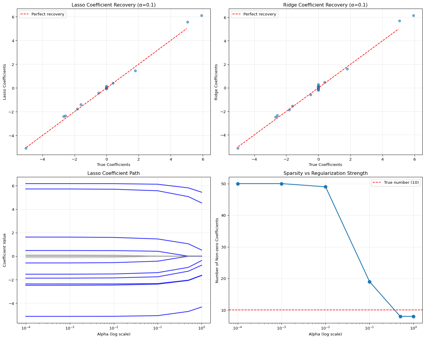
8 Cross-Validation for Optimal Alpha
Use cross-validation to find the optimal regularization parameter.
# Use LassoCV for automatic alpha selection
from sklearn.linear_model import LassoCV

# Define a range of alphas to test
alphas_cv = np.linspace(0.0001, 0.3, 50)

# Perform cross-validation
# cv=5 means 5-fold cross-validation
lasso_cv = LassoCV(alphas=alphas_cv, cv=5, max_iter=10000)
lasso_cv.fit(X_train_scaled, Y_train)

# Get the optimal alpha
optimal_alpha = lasso_cv.alpha_
print(f"Optimal alpha from cross-validation: {optimal_alpha:.4f}")

# Evaluate the model with optimal alpha
Y_test_pred_cv = lasso_cv.predict(X_test_scaled)
test_mse_cv = mean_squared_error(Y_test, Y_test_pred_cv)
test_r2_cv = r2_score(Y_test, Y_test_pred_cv)

print(f"Test MSE with optimal alpha: {test_mse_cv:.4f}")
print(f"Test R² with optimal alpha: {test_r2_cv:.4f}")


# Plot the cross-validation curve
plt.figure(figsize=(10, 6))
plt.errorbar(lasso_cv.alphas_, lasso_cv.mse_path_.mean(axis=1),
            yerr=lasso_cv.mse_path_.std(axis=1),
            label='Mean CV MSE ± 1 std')
plt.axvline(x=optimal_alpha, color='r', linestyle='--',
           label=f'Optimal α = {optimal_alpha:.4f}')
plt.xscale('log')
plt.xlabel('Alpha (log scale)')
plt.ylabel('Mean Squared Error')
plt.title('Cross-Validation Curve')
plt.legend()
plt.grid(True, alpha=0.3)
plt.show()
Optimal alpha from cross-validation: 0.0735
Test MSE with optimal alpha: 1.0446
Test R² with optimal alpha: 0.9910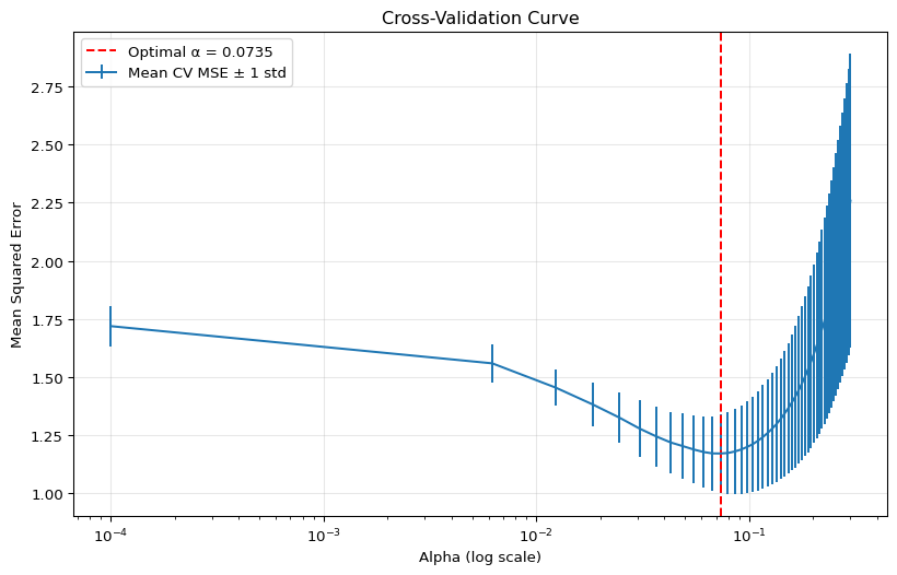
9 Summary
# Create a summary comparison
summary_data = []

# Add Lasso results
for alpha in alphas:
    summary_data.append({
        'Method': 'Lasso',
        'Alpha': alpha,
        'Test MSE': lasso_results[alpha]['test_mse'],
        'Test R²': lasso_results[alpha]['test_r2'],
        'Non-zero Coefficients': lasso_results[alpha]['n_nonzero_coef']
    })

# Add Ridge results
for alpha in alphas:
    summary_data.append({
        'Method': 'Ridge',
        'Alpha': alpha,
        'Test MSE': ridge_results[alpha]['test_mse'],
        'Test R²': ridge_results[alpha]['test_r2'],
        'Non-zero Coefficients': n_features  # Ridge doesn't set coefficients to zero
    })

# Add CV Lasso result
summary_data.append({
    'Method': 'Lasso (CV)',
    'Alpha': optimal_alpha,
    'Test MSE': test_mse_cv,
    'Test R²': test_r2_cv,
    'Non-zero Coefficients': np.sum(lasso_cv.coef_ != 0)
})

summary_df = pd.DataFrame(summary_data)
print("\nModel Comparison Summary:")
print(summary_df)
Model Comparison Summary:
        Method     Alpha  Test MSE   Test R²  Non-zero Coefficients
0        Lasso  0.000100  1.479455  0.987239                     50
1        Lasso  0.001000  1.460491  0.987402                     50
2        Lasso  0.010000  1.300284  0.988784                     49
3        Lasso  0.100000  1.031406  0.991103                     19
4        Lasso  0.500000  3.097040  0.973286                      8
5        Lasso  1.000000  9.088628  0.921605                      8
6        Ridge  0.000100  1.481606  0.987220                     50
7        Ridge  0.001000  1.481570  0.987220                     50
8        Ridge  0.010000  1.481209  0.987224                     50
9        Ridge  0.100000  1.477788  0.987253                     50
10       Ridge  0.500000  1.466591  0.987350                     50
11       Ridge  1.000000  1.461376  0.987395                     50
12  Lasso (CV)  0.073545  1.044583  0.990990                     23
10 Exercises
10.1 Exercise 1: Effect of Sample Size
Modify the code to investigate how the sample size affects Lasso’s ability to recover the true coefficients. Try n_samples = [100, 200, 1000] and plot the feature selection performance.
10.2 Exercise 2: Different Sparsity Levels
Change the number of informative features (n_informative) to see how sparsity affects performance. Try values like 5, 20, 50, and 100.
10.4 Exercise 3: Interpretation
Write a short report (200-300 words) explaining: 1. Why does Lasso perform feature selection while Ridge doesn’t?
In what situations would you prefer Lasso over Ridge?
What are the limitations of Lasso for feature selection?
11 Additional Resources
Submission Instructions: 1. Complete all exercises 2. Add your own analysis and interpretations 3. Submit your completed .qmd file and rendered HTML 4. Include a brief reflection on what you learned